Time series decomposition in R
Time series analysis is one of those scary sounding terms that in reality is very simple. All it means is that you have data where the independent variable is time (seconds, minutes, hours, days, weeks, months, or years) and a dependent that changes over time. Time series analysis is just methods for detecting trends in the dependent variable over time.
The most basic time series analysis is linear regression, which I previously covered here. In this post, I'll discuss time series decomposition. Time series decomposition means that you break a time series into its constituent parts: Trend, seasonal, and random. Seasonal means changes that occur in a regular cycle over the course of a year. Random is random fluctuations within a time series that are neither part of the seasonal pattern nor the trend. I'll demonstrate time series decomposition using Antarctic sea ice data.
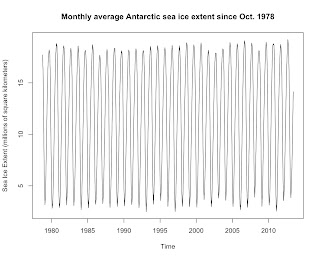
First, a graph of monthly average Antarctic sea ice since satellite records began in October 1978.
And here's the code I used to create it:
Antarctic sea ice is clearly dominated by a seasonal cycle, making it difficult to see any trend in the data. That cycle will also mess up any trend analysis, as it will make the standard errors unnecessarily large, thereby decreasing the chances of detecting significant trends. A linear regression of the raw data gives us this:

The main peak is at 1 year and you can see decreasing harmonics of that cycle at 2 years, 3, years.... Removing the cycle can be done in two ways. The first method is to decompose the data and then subtracting the seasonal component to get seasonally adjusted data.

If you want individual plots of the trend, seasonal, or random components, just type plot(Antarctica.decomp$trend), plot(Antarctica.decomp$seasonal), or plot(Antarctica.decomp$random). Seasonally adjusted data is made by subtracting the seasonal component out of the original time series:
 The trend is clearer although the data is still messy, especially with that large spike in the late 1980s. Calculating the trend by linear regression shows us this:
You can get a moving average from the decomposition data—the trend component is a 12-month moving average, averaging the 6 months prior and the 6 months after the target month. Plotting the trend and fitting a regression line to it is simple:
 This method also removes the random component from the time series in addition to the seasonal cycle, making the overall trend extremely easy to analyze. The overall trend of +16,509 km2 per year is extremely significant (p < 0.00000000000000022).
If you just want to go straight to the moving average without first decomposing the data, you can do so using the SMA command from the TTR package. If you don't already have TTR, download it either via your Packages Installer or via command line:
Update
Just because I know someone will ask, here's the decomposed trend for the Arctic:
 With a trend is -54,533 km2 per year (p < 0.00000000000000022), the Arctic is losing far more sea ice per year than the Antarctic is gaining.
First, a graph of monthly average Antarctic sea ice since satellite records began in October 1978.

And here's the code I used to create it:
Ice = subset(Climate, Time>=1978.75) #create a new data objectA quick note on the second line of code. The "ts" command means simply "create a time series". "Ice$Antarctic.Ice" is the standard way to isolate one single column from a larger data object. The "start = c(1978, 10)" code just tells R that the new time series starts in October 1978 and "frequency" is how many times data is recorded over the course of a year.
Antarctic = ts(Ice$Antarctic.Ice, start = c(1978,10), frequency = 12)
plot(Antarctica, ylab="Sea Ice Extent (millions of square kilometers)", main="Monthly average Antarctic sea ice extent since Oct. 1978")
Antarctic sea ice is clearly dominated by a seasonal cycle, making it difficult to see any trend in the data. That cycle will also mess up any trend analysis, as it will make the standard errors unnecessarily large, thereby decreasing the chances of detecting significant trends. A linear regression of the raw data gives us this:
Antarctica.lm = lm(Antarctica~time(Antarctica)) #time(Antarctica) means extract the time component
summary(Antarctica.lm)
Call:In this analysis, the trend of +13,460 km2 per year is nowhere near statistically significant p = 0.6208. The first step to removing the seasonal cycle is to confirm its existence using Fourier spectral analysis:
lm(formula = Antarctica ~ time(Antarctica))
Residuals:
Min 1Q Median 3Q Max
-9.2403 -5.6873 0.2623 5.1676 7.4690
Coefficients:
Estimate Std. Error t value Pr(>|t|)
(Intercept) -15.29993 54.25622 -0.282 0.778
time(Antarctica) 0.01346 0.02718 0.495 0.621
Residual standard error: 5.568 on 415 degrees of freedom
Multiple R-squared: 0.0005902, Adjusted R-squared: -0.001818
F-statistic: 0.2451 on 1 and 415 DF, p-value: 0.6208
Antarctica.diff = diff(Antarctica) #remove any potential trends by differencing the data
spectrum(Antarctica.diff, method=c("ar"))

Antarctica.decomp = decompose(Antarctica)
plot(Antarctica.decomp)

If you want individual plots of the trend, seasonal, or random components, just type plot(Antarctica.decomp$trend), plot(Antarctica.decomp$seasonal), or plot(Antarctica.decomp$random). Seasonally adjusted data is made by subtracting the seasonal component out of the original time series:
Antarctica.seasonal = Antarctica - Antarctic.decomp$seasonal
plot(Antarctica.season, ylab="Sea ice extent (millions of square kilometers)", main="Seasonally adjusted Antarctic sea ice extent")

Antarctica.season.lm=lm(Antarctica.season~time(Antarctica.season))
summary(Antarctica.season.lm)
Call:Removing the yearly cycle has made detecting the trend in the data much easier. The trend of +16,377 km2 per year is highly significant (p = 0.0000000000005826). However, the seasonally-adjusted method has one major weakness. It assumes that the magnitude of the yearly cycle does not change over time. If the magnitude of the cycle is changing over time (like it is in the Arctic), then seasonally adjusting the data will result in part of the yearly cycle remaining in the data. If that is the case, go straight to a moving average.
lm(formula = Antarctica.season ~ time(Antarctica.season))
Residuals:
Min 1Q Median 3Q Max
-1.15876 -0.26007 -0.01012 0.26456 3.02754
Coefficients:
Estimate Std. Error t value Pr(>|t|)
(Intercept) -21.090252 4.393670 -4.80 2.22e-06 ***
time(Antarctica.season) 0.016377 0.002201 7.44 5.83e-13 ***
---
Signif. codes: 0 ‘***’ 0.001 ‘**’ 0.01 ‘*’ 0.05 ‘.’ 0.1 ‘ ’ 1
Residual standard error: 0.4509 on 415 degrees of freedom
Multiple R-squared: 0.1177, Adjusted R-squared: 0.1156
F-statistic: 55.36 on 1 and 415 DF, p-value: 5.826e-13
You can get a moving average from the decomposition data—the trend component is a 12-month moving average, averaging the 6 months prior and the 6 months after the target month. Plotting the trend and fitting a regression line to it is simple:
Antarctica.trend = lm(Antarctica.decomp$trend~time(Antarctica.decomp$trend))
summary(Antarctica.trend)
plot(Antarctica.decomp$trend, ylab="Sea ice extent (millions of square kilometers)", main="12-month moving average of Antarctic sea ice extent")
abline(Antarctica.trend, lwd=2, col="red")

If you just want to go straight to the moving average without first decomposing the data, you can do so using the SMA command from the TTR package. If you don't already have TTR, download it either via your Packages Installer or via command line:
install.packages(c("TTR"))and follow the prompts. Load TTR into R with
library(TTR)then run the simple moving average command using a 12-month running average and analyze it:
Antarctica.sma = SMA(Antarctica, n = 12)The end result is the nearly the same as using the trend component from decomposition analysis, showing a trend of 16,463 km2 per year (p < 0.00000000000000022). The difference between the decomposition trend and the SMA trend is a slight difference in how SMA calculates the moving average. Whereas decomposition calculates the moving average of the previous and following 6 months, SMA calculates the moving average of the previous 11 months plus the target month.
Antarctica.sma.lm = lm(Antarctica.sma~time(Antarctica.sma))
summary(Antarctica.sma.lm
plot(Antarctica.sma, ylab="Sea ice extent (millions of square kilometers)", main="12-month moving average of Antarctic sea ice extent")
abline(Antarctica.sma.lm, lwd=2, col="red")
Update
Just because I know someone will ask, here's the decomposed trend for the Arctic:


Comments
Post a Comment